
By now you probably already know that Oracle Analytics Cloud (OAC) provides several machine learning (ML) algorithms to support predictive analytics with no coding required. With multiple ML models to choose from in OAC, it is important to know how to compare models. In this blog post we will discuss how to evaluate and compare ML models for the specific task of predicting HR attrition. We will do this by creating, training and testing 3 ML models that are available in OAC using the same training data set for all three models. We will then compare the quality and metrics for each model to see which will work best for our desired end result. We will use a data set related to HR attrition that is freely available for download from Kaggle:
https://www.kaggle.com/pavansubhasht/ibm-hr-analytics-attrition-dataset
This training data set is a ‘labeled’ data set meaning that each row has a value for attrition – either yes or no.
This brings us to some definitions about the two major types of machine learning – Supervised Learning and Unsupervised Learning.
In Supervised Learning, we train a model using a labeled data set. In effect, we give the model the answers and ask it to use these ‘answers’ to infer the rules for predicting a specific value – in this case attrition. Once the model has been trained, it can be used against unlabeled data sets to predict the desired value.
In Unsupervised Learning, the model is trained using an unlabeled data set. In this case the answers are not given to the model. The model is asked to find previously unknown patterns in the data that can be used for clustering, anamoly detection and association mining (eg for market basket analysis).
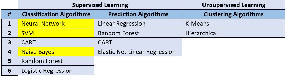
Oracle Analytics Cloud provides algorithms for both Supervised Learning and Unsupervised Learning. Below is a table that lists all the machine learning algorithms available in Oracle Analytics Cloud. The algorithms highlighted in yellow will be used as examples in this blog post. Please note that prediction algorithms are used to predict numeric values while classification algorithms are used to predict non numeric values like attributes, categories, binary values, etc.
Here are the steps we will take:
- Upload the labeled HR attrition data set to OAC and train the Naïve Bayes model
- Analyze and explain the quality and key metrics for the Naïve Bayes model
- Repeat the steps from #1 to train the Neural Network and SVM models
- Analyze the quality and key metrics of the Neural Network and SVM models
- Compare all three models
Upload the Training Data Set and Train the Naïve Bayes Model
Step 1: Upload Labeled Training Data Set to OAC

The second column contains the value for attrition. This is our labeled training data set.
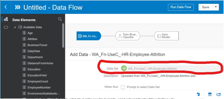
Step 2: Create Data Flow – Add Labeled Training Data Set
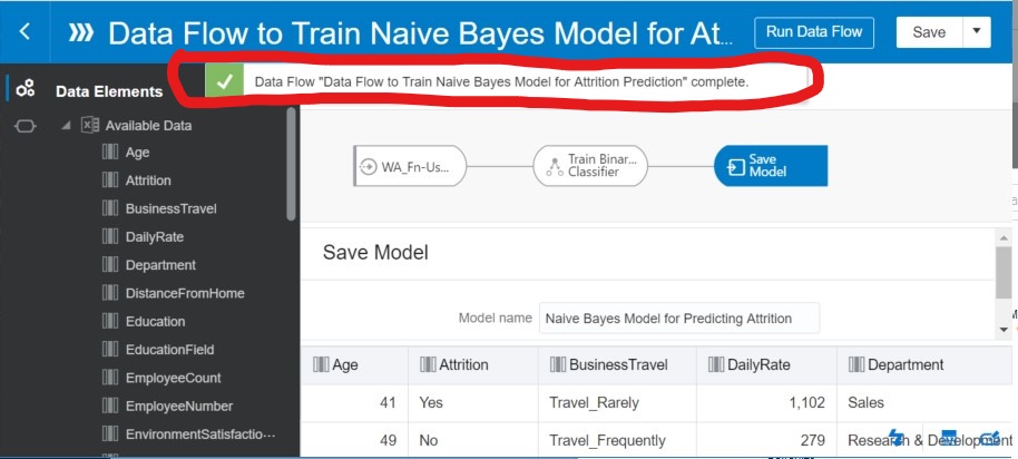
The next step is to create a data flow where we will use this data set to train the model. In the screen below, you can see in the red circled area that the labeled training data set has been added to the data flow.
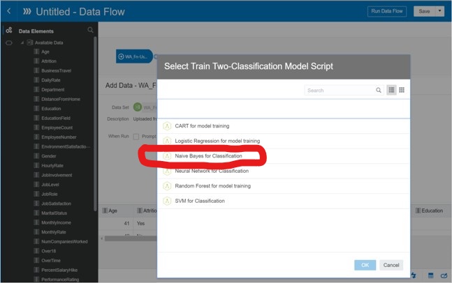
Step 3: Create Data Flow – Select Machine Learning Algorithm
Next we will select the machine learning algorithm to be used to predict attrition. We will be using the ‘Naïve Bayes for Classification’ model.
Step 4: Create Data Flow – Designate Target for Prediction
In this step we need to designate the target column for prediction. You can see in the red circled area that we have selected the column called ‘Attrition’ to be the target for prediction.

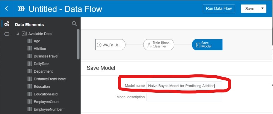
Step 5: Create Data Flow – Give the Training Model a Name
When this data flow is executed it will create a training model. In this next step we give the training model a name (i.e., Naïve Bayes Model for Predicting Attrition).

Guide to Oracle Cloud: 5 Steps to Ensure a Successful Move to the Cloud
Explore key considerations, integrating the cloud with legacy applications and challenges of current cloud implementations.
Step 6: Save and Execute the Data Flow to Create, Train and Test the Model
Now we need to save the data flow and then execute it to ‘train the model’. The model is created by successful execution of the data flow.
Now we have a trained ML model for predicting HR attrition. Next we will analyze the quality and key metrics of this model.
Analyze and Explain the Quality and Key Metrics for the Naïve Bayes Model
When we train a model in OAC we need to define how much of the data set will be used to train the model and how much of the data set will be used to test the model. In this case we chose to use 80% of the data set to train the model and 20% of the data set to test the model.
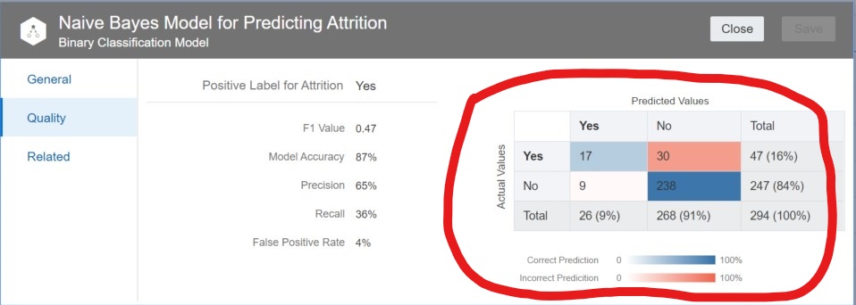
Below is a summary of the results from the testing of the Naïve Bayes model that we just trained. This chart is called a confusion matrix and contains the key metrics that can be used to evaluate the quality of the model and understand how it will behave when used to predict attrition in unlabeled data sets.
Below is an explanation for each of these important, key metrics:
Positive Label: The positive label for attrition in this model is ‘Yes’.
Model Accuracy: This defines how many correct predictions were made by the model as a % of all rows in the test data set. The overall accuracy for this model is 87% – calculated as (238+17)/294.
Precision: Percentage of truly positive predicted instances to total positive instances predicted [17/17+9=65%]. Please note that the denominator for Precision is the total # of positive instances predicted by the model. Precision does not say anything about how many positive instances should have been predicted by the model (E.g., in this case the model predicted a total of 26 positive instances, but there were 47 actual positive instances – so the model did not address a large number of truly positive instances). Although Precision is an important metric, a model with the highest Precision is not necessarily the best model.
Recall: Percentage of truly positive predicted instances to total actual positive instances [17/17+30=36%]. Recall is important to analyze in conjunction with Precision because Recall addresses how many truly positive predictions should have been made by the model. It will tell you whether the model will correctly address just a thin slice of your data set or whether the model will have broad coverage. Just like with Precision, a model with a high Recall is not necessarily the best model.
F1 Value: This is the harmonic mean (reciprocal of the arithmetic mean of the reciprocals) of Precision and Recall [2/((1/.65)+(1/.36)) =.47]. The F1 value is a measure of the balance between Precision and Recall. A measure of 1 for F1 means perfect Precision and Recall (which is very rare).
False Positive Rate: Percentage of false positive instances to total actual negative instances [9/247=4%]. A low false positive rate is required for Precision to be high.
Train the Neural Network and SVM Models
I will repeat the same steps that were used to train the Naïve Bayes model to train the Neural Network and SVM models. To do so, in Step 3 above I will select either Neural Network as the algorithm instead of Naïve Bayes.
Analyze the Quality and Key Metrics of the SVM and Neural Network Models
Having trained the Neural Network and SVM models, we can now look at the confusion matrix for each one.
Below is the confusion matrix for the Neural Network model.

Let’s analyze the quality and key metrics of this Neural Network model in relation to the Naïve Bayes model:
Model Accuracy: 80% – this is a little less than the 87% for the Naïve Bayes model.
Precision: 38% – this is significantly lower than the 65% of the Naïve Bayes model.
Recall: 36% – this is the same as the Naïve Bayes model. Unfortunately, although Precision is less in this model, there is no offsetting benefit in the form of a higher Recall %.
False Positive Rate: 11% – this is higher than the Naïve Bayes model but with no increase in Recall.
In comparison to the Naïve Bayes model, the Neural Network model does not offer any significant advantages. Precision is much lower than Naïve Bayes with no offsetting increase in Recall. Also, the false positive rate is higher – again without any increase in Recall.
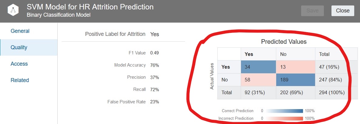
Now let’s take a look at the metrics for the SVM model. Below is the confusion matrix for the SVM model.
Let’s analyze the quality and key metrics of this SVM model in relation to the Naïve Bayes model:
Model Accuracy: 76% – this is less than the 87% of the Naïve Bayes.
Precision: 37% – this is significantly lower than the 65% of the Naïve Bayes model.
Recall: 72% – this is double the 36% of the Naïve Bayes model and the Neural Network model. This SVM model had more truly positive predictions than both the Naïve Bayes model and the Neural Network model. It covers more of the data set in terms of accurate predictions than the Naïve Bayes and Neural Network models.
False Positive Rate: 23% – this is higher than both the Naïve Bayes model and the Neural Network model. So the cost (so to speak) of a higher Recall % with the SVM model is a higher false positive rate.
Compare All Three Models
Below is a chart that compares all three models.

In order to decide which model would be best for predicting attrition we have to define what is important. Since we are predicting attrition, we don’t want to miss any situations where someone is at risk of leaving the company. To say this another way, we want to maximize the Recall %. This is the same as saying we want a model that accurately predicts as many truly positive cases as possible.
The other criteria to analyze is the impact of false positives vs false negatives. With regard to attrition, a false negative would mean that we erroneously conclude that a person is not at risk of leaving the company. We could potentially lose the opportunity to prevent such a person from leaving. A false positive would mean we might take some action to retain a person who was not actually at risk of leaving the company in the first place.
Final Conclusion
Although there is no absolute correct answer (depends on what is important to each company), if we believe the consequence of a false negative (someone leaving the company) is more detrimental than the consequence of a false positive (giving attention to someone who maybe does not need it), and we are willing to ‘put up with’ the false positives, then the SVM model may be the correct model to use.